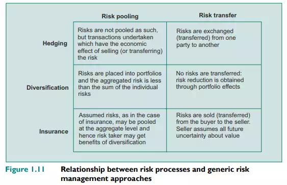
At the level of the economy, risk management makes use of basically two approaches to modifying the level of risk, either risk pooling (sharing) or risk transfer. At the aggregate level the total amount of risk in the economy cannot be reduced, but its economic consequences can be modified through sharing its consequences or transferring the risk to another party better able to accept the consequences of the risk. With risk pooling, or risk sharing, the effects of risks are spread among all market participants. Insurance is an example where losses are shared among the pool of insured parties. Risk transfer involves reassigning the risk to another party for a fee. For instance, many industrial and commercial firms transfer their foreign exchange exposures to banks by buying forward foreign exchange contracts. The bank then manages the resultant risks. In addition, while the process of financial risk management activities may seem complex – and this often serves to mask the inherent benefits from undertaking the process – this same apparent complexity also hides the fact that the risk management process has three generic approaches, namely hedging, diversification and insurance.

Hedging leads to the elimination of risk through its sale in the market, either through cash or spot market transactions or through a transaction, such as a forward, future or swap, that represents an agreement to sell the risk in the future. For instance, the UK-domiciled exporter being paid in euros when the goods are delivered at some date in the future can hedge this exchange rate risk by entering into a forward exchange agreement (with a bank) to sell the euros it will receive at a fixed price and receive a known amount of British pounds rather than leave the result to unknown fluctuations in the exchange rate. Diversification reduces risk by combining less than perfectly correlated risks into portfolios. For instance, while individual borrowers from a bank each represent a significant element of credit risk, for the depositors at the average bank there are virtually no concerns about credit risk.* Insurance involves paying a fee to limit risk in exchange for a premium. For example, one has only to consider the benefits to be derived from paying a fixed premium to protect against property damage or loss, or for life assurance, in the traditional insurance contract. In doing so, the insurer, usually an insurance company, takes on the risk of unknown future losses. Figure 1.11 illustrates how the relationship between risk modification (through risk pooling and risk transfer) and the generic risk management approaches might work. Any risk management transaction can be mapped onto this template.

All definitions of risk share two common factors: the indeterminacy of the outcome and the chance of loss. That the result is not a foregone conclusion is implicit in any concept of risk: the outcome must be in question. For a risk to exist, there must be at least two possible outcomes. If we were to know for sure that a loss was the result, there would be no risk; we would avoid the situation or accept the consequences. For instance, when we buy a new car, we know that the value of the car will depreciate with age and use: here the outcome is (more or less) certain, and there is no risk. The other element of risk is that at least one outcome is unexpected and undesirable. This is a loss in the sense that something of value is lost or that the gain in value is less than what it was possible to achieve. For instance, an asset whose return – or appreciation in value – is less than an alternative would result in an opportunity loss. That is why the depreciation you experience when you own a car is not a risk. While it is undesirable, it is not unexpected. It follows from knowing that the asset, a car in this case, will lose value over time as it wears out.

Bryan Wynne (1992) proposes a four-level stratification:

1. risk, where probabilities are known;

2. uncertainty, where the main parameters are known but quantification is suspect;

3. indeterminacy, where the causation or risk interactions are unknown.

4. ignorance, where we don’t know what we don’t know. This refers to the risks that have, so far, escaped detection or have not manifested themselves.

We can define risk as the set of outcomes for a given decision to the occurrence of which outcomes we may assign a probability. Uncertainty implies that it is not possible to quantify the extent of the hazard. It follows, therefore, that with risk the outcome is unknown but we can somehow define the boundaries of the possible set of outcomes. Risk can be quantified, whereas uncertainty cannot. While we can make great play of the difference between risk and uncertainty, the two are often used interchangeably. In so far as certain unexpected outcomes cannot be easily quantified, they are uncertain rather than ‘risky’ under this definition. This is clear when we consider the relationship between risk and exposure, two terms that are often used interchangeably. Risk is the probability of a loss; exposure is the possibility of loss. While the two terms are often used interchangeably, risk arises from an exposure. Hence, as shown by the example companies given in Section 1.1.6, a firm’s line of business creates exposures that are risky and therefore need to be managed.

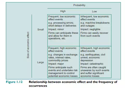
We can further refine our thinking by considering events that are common but lead to small losses and events that are infrequent but lead to high losses. This latter category is often the most troublesome, since occurrences are infrequent and difficult to anticipate. We can hence categorise risk and frequency as shown in Figure 1.12.

To be able to assess risks involves breaking the overall risk down into its component parts. The basic risk paradigm, as shown in Figure 1.13, based on MacCrimmon and Wehrung (1986), is a decision problem where there is a choice between only two outcomes: a certain outcome (X: often but not exclusively the status quo) and an uncertain outcome that is the result of two possible events, each of which has a certain chance or probability of occurring, where one outcome produces a gain (G) and the other a loss (L). The financial equivalents to this risk model are the Sharpe–Lintner Capital Asset Pricing Model (CAPM), as developed by Sharpe (1964), Lintner (1965) and others, and Arbitrage Pricing Theory (APT), as proposed by Ross (1976).