
To see how we might estimate risk, think of the situation when we throw two dice with the normal 1 through 6 on each of the faces. There are 36 possible combinations with values ranging from 2 (snake eyes, or double 1) through to 12 (double 6). The likelihood of any number on a given dice is 1/6. But a little thought will show that the likelihood of both dice giving a 1, for instance, is 1/6 × 1/6 or 1/36. So extreme values of 2 and 12 are unlikely. A number such as 7 (which is also the expected outcome) has a much higher likelihood, since a number of different combinations of values can add up to 7: 1 + 6; 2 + 5; 4 + 3 (this can occur in six different combinations when we throw two standard dice). The likelihood of obtaining a value for the two dice of 7 is in fact 6/36 or 1/6. For risk management purposes, to determine just how much risk there is involved, we want to know the possible deviation from the expected outcome. To know this, we need to know the distribution of the outcomes. A histogram of the possible values of the two dice and their frequency is given in Figure 1.14.
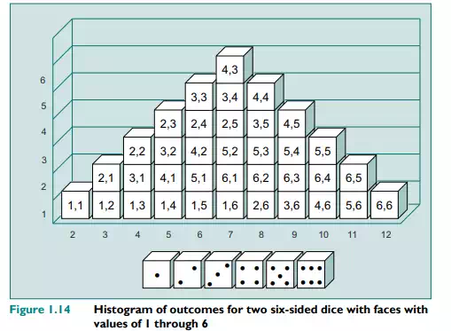
A spreadsheet version of this figure is available on the EBS course website. In quantifying the risk, we can first calculate the expected value of the two dice. This is 7. Given this, we can now calculate the variance and standard deviation using the quantification formula:
This gives a value for the variance of 5.83, and for the standard deviation, which is the square root of the variance (√5.83), of 2.42. Now let us look at another example of dice similar to the one above, except in this case the dice are what are known as average dice. These dice have values that are closer to the average of a normal dice (which is 3.5) and have faces numbered 2, 3, 3, 4, 4 and 5. The histogram of outcomes is given in Figure 1.15. A comparison of Figure 1.14, for the normal two dice outcomes, and that of Figure 1.15, for two average dice outcomes, shows that the spread of possible outcomes and their likelihood is very different. Whereas with the normal two dice the average value, 7, is expected in 6/36 cases, with the average dice it occurs in 10/36 cases. Also, the likelihood of getting outcomes close to the average (namely 6 or 8) is much higher in the case of the average dice.
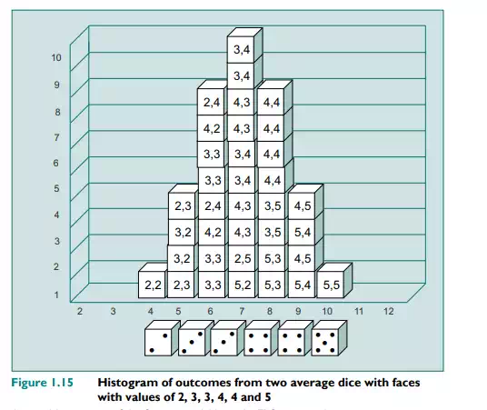
As with the normal dice, we can calculate the spread using the variance equation. This gives 1.83 for the average dice variance and 1.35 for its standard deviation. Hence, the dice are missing the extreme values of 1 and 6. In the language of risk management, we would say that an average dice is less risky than a conventional one, since the dispersion of values is smaller. The maximum range for a standard six-sided dice is 1 to 6, or a variance of 5 between the extreme outcomes. For the average dice, the range is 2 to 5, or a range of 3. Both dice have the same expected value. Hence, following our definition of risk, the standard dice is the riskier.
What the two statistics do is to provide us with a metric for measuring the relative riskiness of the two situations. A glance at the two histograms will immediately show there is a greater chance of significantly divergent outcomes for the normal dice. For instance, the probability of getting an outcome more than two values away from the mean (in either direction) – i.e. values that are less than 5 (4, 3, 2) and more than 9 (10, 11, 12) – for the two cases is:
Normal dice: 0.33
Average dice: 0.06
We can use the variance or standard deviation statistic, therefore, as an objective measure of risk for comparison purposes.
As previously stated, the ris